此篇總結 透視 XGBoost 系列，建議系列閱讀順序為

1. 透視 XGBoost(1) 圖解 Regression
2. 透視 XGBoost(2) 圖解 Classification
3. 透視 XGBoost(3) 蘋果樹下的 objective function
4. 透視 XGBoost(4) 神奇 optimization 在哪裡？

XGBoost 不只在算法上的改造，真正讓 XGBoost 大放異彩的是與工程優化的結合，這讓 XGBoost 在工業上可以應用於大規模數據的處理。

• Approximate Greedy Algorithm
• Weighted Quantile Sketch & Parallel Learning
• Sparsity-Aware Split Finding
• System Design

Approximate Greedy Algorithm

XGBoost 有兩種 split finding 策略，Exact Greedy and Approximate Greedy

data sample 量小的情況下， XGB tree 在建立分支時，會逐一掃過每個可能分裂點 (已對特徵值排序) 計算 similarity score 跟 gain， 即是 greedy algorithm。

greedy algorithm 會窮舉所有可能分裂點，因此能達到最準確的結果，因為他把所有可能的結果都看過一遍後選了一個最佳的。

但如果 data sample 不僅數量多 (row)，特徵維度也多 (columns)，採用 greedy algorithm，雖然準確卻也沒效率。

XGBoost General Objective Function

XGboost 是 gradient boosting machine 的一種實作方式，xgboost 也是建一顆新樹 $f_m(x)$ 去擬合上一步模型輸出 $F_{m-1}(x)$ 的 $\text{residual}$

$$\begin{aligned} F_m(x) & = F_{m-1}(x) + f_m(x) \\ F_{m-1}(x) &= F_0(x) + \sum_{i=1}^{m-1}f_{i}(x) \end{aligned}$$

不同的是， XGBoost 用一種比較聰明且精準的方式去擬合 residual 建立子樹 $f_m(x)$

此篇首先推導了 XGBoost 的通用 Objective Function，然後解釋為何 second order Taylor expansion 可以讓 XGBoost 收斂更快更準確

XGBoost’s Objective Function

XGBoost 的 objective function 由 loss function term $l(y_i, \hat{y_i})$ 和 regularized term $\Omega$ 組成

$$\begin{aligned} \mathcal{L}& = [\sum_i^n l(y_i, \hat{y_i}) ] + \sum_{m}\Omega({f_m}) \end{aligned}$$

• $\mathcal{L}$ 表 objective function
• $l(y_i, \hat{y_i})$ 表 loss function
  • in regression, loss function $l(y_i, \hat{y_i})$ commonly use square error
  • in classification，最大化 log likelihood 就是最小化 cross entropy
• $f_m$ 表 第 m 步 XGB tree
• regularized term $\Omega$ 跟 XGB tree $f_m(x)$ leaf node number $T_m$ 與 each leaf node output $\gamma$ 有關
  • $\Omega(f_m) = \tau T_m + \cfrac{1}{2}\lambda \lVert \gamma \rVert ^2$
    • $\lambda$ is a regularization parameter
    • $T_m$ is the number of leaf in tree $f_m$
    • $\tau$ 表對 $T_m$ 的 factor

在 第 $m-1$ 步建完 tree $f_{m-1}$時，total cost 為

$$\begin{aligned} \mathcal{L}^{(m-1)}& = [\sum_{i=1}^n l(y_i, \hat{y_i}^{(m-1)}) ] + \Omega({f_{(m-1)}}) \\ &=[\sum_{i=1}^n l(y_i, F_{(m-1)}(x_i) ] + \Omega({f_{(m-1)}}) \end{aligned} \tag{4}$$

• $\hat{y_i}^{(m-1)}$ 表 $F_{m-1}(x_i)$ 預測值
• $f_{m-1}$ 表 第 $m-1$ 步建立的 XGB tree

進入第 $m$ 步，我們建一顆新樹 $f_m(x)$ 進一步減少 total loss，使得 $\mathcal{L}^{(m)}< \mathcal{L}^{(m-1)}$ ， 則 $m$ 步 cost function 為

$$\begin{aligned} \mathcal{L}^{(m)}& = [\sum_i^n l(y_i, F_{m-1}(x_i) + f_m(x_i)) ] + \Omega({f_{(m)}}) < \mathcal{L}^{(m-1)} \end{aligned} \tag{5}$$

現在要找出新樹 $f_m(x_i)$ 的每個 leaf node 輸出能使式 (5) $\mathcal{L}^{(m)}$ 最小

$$\gamma_{j,m} = argmin_\gamma \sum_{x_i \in R_{j,m}} [l(y_i, F_{m-1}(x_i) + \gamma)] + \Omega({f_{(m)}}) \tag{6}$$

• $j$ 表 leaf node index
• $m$ 表第 $m$ 步
• $\gamma_{j,m}$ $m$ 步 $f_m$ 第 $j$ 個 leaf node 的輸出值
• $R_{jm}$ 表 $m$ 步 第 $j$ 個 leaf node，所包含的 data sample $x$ 集合

當 loss function $l(y, \hat{y})$ 為 square error 時，求解式 (6) 不難，但如果是 classification problem 時，就變得很棘手。

所以 GBDT 對 regression problem 與 classification problem 分別用了兩種不同方式求解極值，求出 leaf node 的輸出

• for regression ：硬解 derivative ，因爲 MSE 的 derivative 簡單 一步步透視 GBDT Regression Tree
• for classification: use the Second Order Tayler Approximation 化簡 loss function 一步步透視 GBDT Classifier

Second Order Tayler Approximation 的步步逼近

XGBoost 直接以 Second Order Tayler Approximation 處理 classification 跟 regression 的 loss function part $l(y,\hat{y})$

式(5) 的 loss function part 在 $\hat{y}^{m-1}(x_i)$ 附近展開:

$$\begin{aligned} l(y,\hat{y}^{(m-1)} + f_m(x)) \approx & \quad l(y, \hat{y}^{(m-1)}) + [\cfrac{d}{d \ \hat{y}^{(m-1)}} \ l(y, \hat{y}^{(m-1)})]f_m(x) + \cfrac{1}{2}[\cfrac{d^2}{d \ (\hat{y}^{(m-1)})^2} \ l(y, \hat{y}^{(m-1)})] f_m(x)^2 \\ & = l(y, F_{m-1}(x)) + [\cfrac{d}{d \ F_{m-1}} \ l(y, F_{m-1})]f_m(x) + \cfrac{1}{2}[\cfrac{d^2}{d \ F_{m-1}^2} l(y, F_{m-1})] f_m(x)^2 \\ &= l(y, F_{m-1}(x)) + gf_m(x) + \cfrac{1}{2}hf_m(x)^2 \end{aligned}\tag{7}$$

• $\hat{y}^{(m-1)}$ 為 XGB 在 $m-1$ 步的 prediction $F_{m-1}(x)$
• $g = \cfrac{d}{d \ F_{m-1}} \ l(y, F_{m-1})$
• $h = \cfrac{d^2}{d^2 \ F_{m-1}} l(y, F_{m-1})$

將式 (7) 代入式(5)：

$$\begin{aligned} \mathcal{L}^{(m)}& \approx \ [ \sum_i^n(l(y_i, \hat{y}^{(m-1)}_i) +g_if_m(x_i) + \cfrac{1}{2}h_if_m(x_i)^2 ] + \Omega({f_{m}}) \end{aligned} \tag{8}$$

• $g_i$ 為 first derivative of loss function related to data sample $x_i$
• $h_i$ 為 second derivative of loss function related to data sample $x_i$
• $f_m(x_i)$ 為 $x_i$ 在 XGB tree $f_m(x)$ 的 output value

式 (8) 即 XGBoost 在 $m$ 步的 cost function

$\mathcal{L}^{(m)}$ 束手就擒

Second Order Tayler Approximation 逼近 loss function $l(y, \hat{y})$後 ，對 $\mathcal{L}^{(m)}$ 求 $\gamma_{j,m}$ 極值，就變得容易多了

先將 regularization term $\Omega({f_{m}})$ 展開代入式 (8)，並拿掉之後對微分沒影響的常數項 $l(y_i, \hat{y}^{(m-1)}_i)$

$$\begin{aligned} \mathcal{\tilde{L}}^{(m)}& = [ \sum_i^n( g_if_m(x_i) + \cfrac{1}{2}h_if_m(x_i)^2) ] + [\tau T_m + \cfrac{1}{2}\lambda \sum^T_{j} \gamma_{m,j}^2] \\ &= \sum^{T_m}_{j=1}[(\sum_{i \in R_{m,j}}g_i) \gamma_{j,m} + \cfrac{1}{2}(\sum_{i \in R_{j,m} }h_i + \lambda)\gamma_{j,m}^2] + \tau T_m \end{aligned} \tag{9}$$

• $T_m$ is the number of leaf in tree $f_m$
• $\tau$ 表對 $T_m$ 的 factor
• $\gamma_{j,m}$ 表 $m$ 步 XGB tree $f_m$ 第 $j$ 個 leaf node 的輸出值
• $R_{m,j}$ 表 leaf node j 下的 data sample $x$ 集合
• 第一個等式到第二個等式 : 從原本遍歷所有 data sample $x$ 到遍歷所有 leaf node $R_{m,j}$ 下的 data sample

式 (9) 對 $\gamma_{j,m}$ 微分取極值

$$\cfrac{d}{d \ \gamma_{j, m}} \mathcal{\tilde{L}}^{(m)} = \sum^{T_m}_{j=1}[(\sum_{i \in R_{m,j} }g_i) + (\sum_{i \in R_{j,m}}h_i)\gamma_{j,m}] = 0 \tag{10}$$

對於已經固定結構了 tree $f_m(x)$，式 (10) leaf node $j$ 的 output value $\gamma_{j,m}$ 為

$$\gamma_{j,m}^*=- \cfrac{\sum_{i\in R_{j,m}} g_i}{\sum_{i \in R_{j,m}}h_i + \lambda} \tag{11}$$

• $g_i$ 為 first derivative of loss function related to data sample $x_i$ : $g_i = \cfrac{d}{d \ F_{m-1}} \ l(y_i, F_{m-1}(x_i))$
• $h_i$ 為 second derivative of loss function related to data sample $x_i$: $h_i = \cfrac{d^2}{d \ F_{m-1}^2} l(y_i, F_{m-1}(x_i))$

將 式(11) $\gamma_{j,m}^*$ 代回 式 (9)，即 objective function 的極值

$$\begin{aligned} \mathcal{\tilde{L}}^{(m)} &= \sum^{T_m}_{j=1}[(\sum_{i \in R_{m,j}}g_i) \gamma_{j,m} + \cfrac{1}{2}(\sum_{i \in R_{j,m} }h_i + \lambda)\gamma_{j,m}^2] + \tau T_m \\ &=\sum^{T_m}_{j=1}[-(\sum_{i \in R_{j,m}}g_i)\cfrac{\sum_{i\in R_{j,m}} g_i}{\sum_{i \in R_{j,m}}h_i + \lambda} + \cfrac{1}{2}(\sum_{i \in R_{j,m} }h_i + \lambda)(\cfrac{\sum_{i\in R_{j,m}} g_i}{\sum_{i \in R_{j,m}}h_i + \lambda})^2 ] + \tau T_m \\ & = \sum^{T_m}_{j=1}[-\cfrac{(\sum g_i)^2}{\sum h_i + \lambda} + \cfrac{1}{2} \cfrac{(\sum g_i)^2}{\sum h_i + \lambda}] + \tau T_m \\ & = -\cfrac{1}{2} \sum^{T_m}_{j=1}[\cfrac{(\sum g_i)^2}{\sum h_i + \lambda} ] + \tau T_m \end{aligned} \tag{12}$$

總結

XGBoost 通用 Objective Function

$$\begin{aligned} \mathcal{\tilde{L}}^{(m)} &= \sum^{T_m}_{j=1}[(\sum_{i \in R_{m,j}}g_i) \gamma_{j,m} + \cfrac{1}{2}(\sum_{i \in R_{j,m} }h_i + \lambda)\gamma_{j,m}^2] + \tau T_m \end{aligned}$$

• $g_i$ 為 first derivative of loss function related to data sample $x_i$ : $g_i = \cfrac{d}{d \ F_{m-1}} \ l(y_i, F_{m-1}(x_i))$
• $h_i$ 為 second derivative of loss function related to data sample $x_i$: $h_i = \cfrac{d^2}{d \ F_{m-1}^2} l(y_i, F_{m-1}(x_i))$
• $T_m$ is the number of leaf in tree $f_m$
• $\tau$ 表對 $T_m$ 的 factor
• $\gamma_{j,m}$ 表 $m$ 步 XGB tree $f_m$ 第 $j$ 個 leaf node 的輸出值

Optimal Output of Leaf Node $j$

$$\gamma_{j,m}^*=- \cfrac{\sum_{i\in R_{j,m}} g_i}{\sum_{i \in R_{j,m}}h_i + \lambda}$$

Optimal Value of Objective Function

$$\mathcal{\tilde{L}}^{*(m)} = \cfrac{1}{2} \sum^{T_m}_{j=1}[\cfrac{(\sum g_i)^2}{\sum h_i + \lambda} ] + \tau T_m$$

Why does Approximation with Taylor Expansion Work?

Traditional Gradient Decent

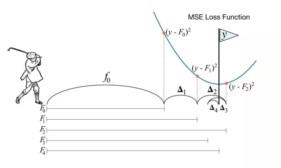
當我們在做 gradient decent 時，我們是在嘗試 minimize a cost function $f(x)$，然後讓 $w^{(i)}$ 往 negative gradient 的方向移動

$$w^{(i+1)} =w^{(i)} - \nabla f(w^{(i)})$$

但 gradient $\nabla f(w^{(i)})$ 本身只告訴我們方向，不會告訴我們真正的 the minimum value，我們得到的是每步後盡量靠近 the minimum value 一點，這使的我們無法保證最終到達極值點

同樣的表達式下的 gradient boost machine 也相似的的問題

$$F_m(x) = F_{m-1}(x) + \nu f_{m}(x)$$

傳統的 GBDT 透過建一顆 regression tree $f_m(x)$ 和合適的 step size $\nu$ (learning rate) 擬合 negative gradient 往低谷靠近，可以說 GBDT tree $f_m(x)$ 本身就代表 loss function 的 $\text{negative graident}$ 的方向

Better Gradient Decent: Newton’s Method

Newton’s method 是個改良自 gradient decent 的做法。他不只單純考慮了 gradient 方向 (即 first order derivative) ，還多考慮了 second order derivative 即所謂 gradient 的變化趨勢，這他更精準的定位極值的方向

$$w^{(i+1)} = w^{(i)} - \cfrac{\nabla f(w^{(i)})}{\nabla ^2f(w^{(i)})} = w^{(i)} - \cfrac{\nabla f(w^{(i)})}{\text{Hess}f(w^{(i)})}$$

XGBoost 引入了 Newton’s method 思維，在建立子樹 $f_m(x)$ 不再單純只是 $\text{negatvie gradient}$ 方向 (即 first order derivative) ，還多考慮了 second order derivative 即 gradient 的變化趨勢，這也是為什麼 XGBoost 全稱叫 Extreme Gradient Boosting

$$f_m(x_i) = \gamma_{j,m}=- \cfrac{\sum_{i\in R_{j,m}} g_i}{\sum_{i \in R_{j,m}}h_i + \lambda}$$

• $\gamma_{j,m}$ 表 $m$ 步 XGB tree $f_m$ 第 $j$ 個 leaf node 的輸出值
• $g_i$ 為 first derivative of loss function related to data sample $x_i$
• $h_i$ 為 second derivative of loss function related to data sample $x_i$

而 loss function $l(y_i,\hat{y_i})$ 會因不同應用: regression , classification, rank 而有不同的 objective function，並不一定存在 second order derivative，所以 XGBoost 利用 Taylor expansion 藉由 polynomial function 可以逼近任何 function 的特性，讓 loss function 在 $f_m(x_i)$ 附近存在 second order derivative

$$\begin{aligned} l(y,\hat{y}^{(m-1)} + f_m(x)) \approx l(y, F_{m-1}(x)) + gf_m(x) + \cfrac{1}{2}hf_m(x)^2 \end{aligned}$$

可以說，XGBoos tree 以一種更聰明的方式往 the minimum 移動

總結

• 一般 GBDT 用 regression tree 擬合 residuals，本質上是往 negative gradient 方向移動
• XGBoost tree $f_m(x)$ 擬合 residuals，同時考慮 gradient 的方向和 gradient 變化趨勢，這讓他朝 optimal value 移動時顯得更加聰明有效
  • gradient 的方向： first order derivative
  • gradient 變化趨勢： second order derivative

Reference

• Chen, T., & Guestrin, C. (2016). XGBoost: A scalable tree boosting system. Proceedings of the ACM SIGKDD International Conference on Knowledge Discovery and Data Mining, 13-17-Augu, 785–794. https://doi.org/10.1145/2939672.2939785

XGBoost Part 1 (of 4): Regression

XGBoost Part 3 (of 4): Mathematical Details

• Tayler expansion
  • XGBoost Loss function Approximation With Taylor Expansion https://stats.stackexchange.com/questions/202858/xgboost-loss-function-approximation-with-taylor-expansion
  • https://en.wikipedia.org/wiki/Taylor_series#Approximation_and_convergence
  • https://en.wikipedia.org/wiki/Taylor’s_theorem

TL;DR

• XGBoost 與 GBDT 相比，同樣都是擬合上一步 $F_{m-1}(x)$ 預測值的 residual 。不同的是 XGBoost 在擬合 residual 時更為聰明有效，他有自己衡量分裂增益 gain 的方式去擬合 residual 建立 XGB tree $f_m(x)$

$$Gain = Left_{\text{similarity}} + Right_{\text{similarity}} - Root_{\text{similarity}} \tag{1}$$

• 分裂增益 gain ，的背後原理可以透過 XGBoost 通用 objective function 並填入 classification/regression/rank/etc.. 各自的 loss function 後推導出的 $\text{first derivative of loss function} = g_i \quad \text{and} \quad \text{second derivative of loss function} = h_i$
• XGBoost 的 通用 objective function 由兩部份組成
  • first part is loss function，根據不同任務有不同的 loss function
  • second part is regularization term 防止 overfitting，限制 leaf node 輸出值大小 和 leaf nodes 的總數

Introduction

XGBoost

XGboost 是 gradient boosting machine 的一種實作方式，xgboost 也是建一顆新樹 $f_m(x)$ 去擬合上一步模型輸出 $F_{m-1}(x)$ 的 $\text{residual}$

$$\begin{aligned} F_m(x) & = F_{m-1}(x) + f_m(x) \\ F_{m-1}(x) &= F_0(x) + \sum_{i=0}^{m-1}f_{m-1}(x) \end{aligned}$$

不同的是，Xgboost 做了大量運算和擬合的優化，這讓他比起傳統 GBDT 更為高效率與有效

TL;DR

• 訓練完的 GBDT 是由多棵樹組成的 function set $f_1(x), …,f_{M}(x)$
  • $F_M(x) = F_0(x) + \nu\sum^M_{i=1}f_i(x)$
• 訓練中的 GBDT，每棵新樹 $f_m(x)$ 都去擬合 target $y$ 與 $F_{m-1}(x)$ 的 $residual$，也就是 $\textit{gradient decent}$ 的方向
  • $F_m(x) = F_{m-1}(x) + \nu f_m(x)$
• GBDT classifier 常用的 loss function 為 cross entropy
• classifier $F(x)$ 輸出的是 $log(odds)$，但衡量 $residual$ 跟 $probability$ 有關，得將 $F(x)$ 通過 $\textit{sigmoid function }$ 獲得 probability
  • $p = \sigma(F(x))$

GBDT 簡介在 一步步透視 GBDT Regression Tree

直接進入正題吧

TL;DR

• 訓練完的 GBDT 是由多棵樹組成的 function set $f_1(x), …,f_{M}(x)$

  • $F_M(x) = F_0(x) + \nu\sum^M_{i=1}f_i(x)$

• 訓練中的 GBDT，每棵新樹 $f_m(x)$ 都去擬合 target $y$ 與 $F_{m-1}(x)$ 的 $residual$，也就是 $\textit{gradient decent}$ 的方向

  • $F_m(x) = F_{m-1}(x) + \nu f_m(x)$

Golf Boosting