一步步透視 GBDT Regression Tree

TL;DR

• 訓練完的 GBDT 是由多棵樹組成的 function set $f_1(x), …,f_{M}(x)$

  • $F_M(x) = F_0(x) + \nu\sum^M_{i=1}f_i(x) $

• 訓練中的 GBDT，每棵新樹 $f_m(x)$ 都去擬合 target $y$ 與 $F_{m-1}(x)$ 的 $residual$，也就是 $\textit{gradient decent}$ 的方向

  • $F_m(x) = F_{m-1}(x) + \nu f_m(x)$

結論說完了，想看數學原理請移駕 背後的數學，想看例子從無到有生出 GBDT 的請到 Algorithm - step by step ，想離開得請按上一頁。

GBDT 簡介

GBDT-regression tree 簡單來說，訓練時依序建立 trees $\{ f_1(x), f_2(x), …. , f_M(x)\}$，每顆 tree $f_m(x)$ 都站在 $m$ 步前已經建立好的 trees $f_1(x), …f_{m-1}(x)$ 的上做改進。

所以 GBDT - regression tree 的訓練是 sequentially ，無法以並行訓練加速。

我們把 GBDT-regression tree 訓練時第 $m$ 步的輸出定義為 $F_m(x)$，則其迭代公式如下:

$$F_m(x) = F_0(x) + \nu\sum^m_{i=1}f_i(x) = F_{m-1}(x) + \nu f_m(x)$$

• $\nu$ 為 learning rate

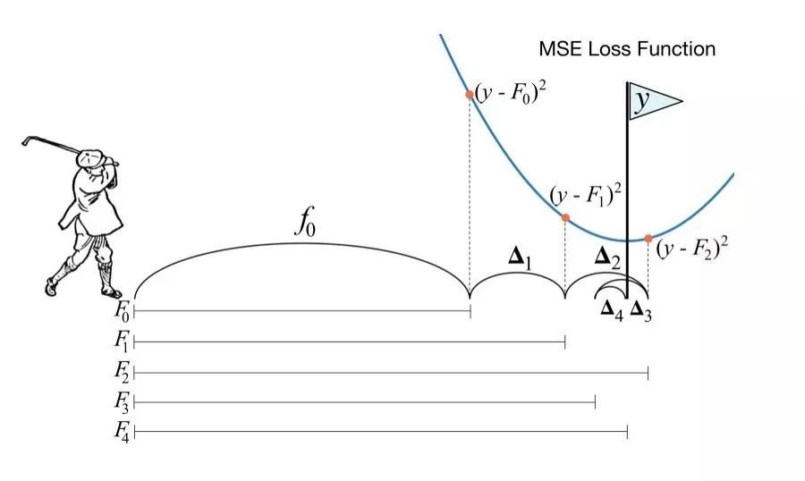
GBDT 訓練迭代的過程可以生動的比喻成 playing golf，揮這一杆 $F_m(x)$ 前都去看 “上一杆 $F_{m-1}(x)$ 跟 flag y 還差多遠” ，再揮杆。

差多遠即 residual 的概念：

$$\textit{residual = observed - predicted}$$

因此可以很直觀的理解，GBDT 每建一顆新樹，都是基於上一步的 residual

GBDT Algorithm - step by step

Algorithm 參考了 statQuest 對 GBDT 的講解，連結放在 reference，必看！

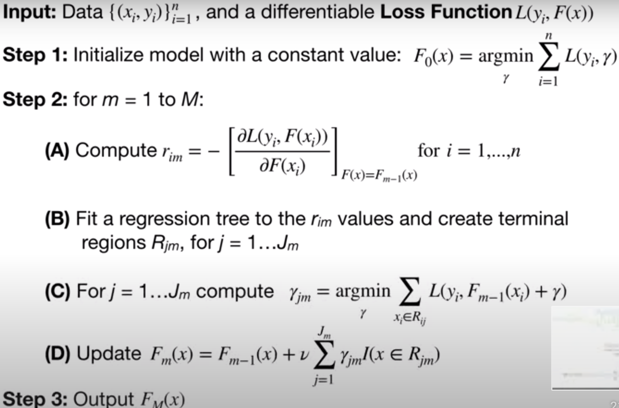
GBDT-regression tree 擬合 algorithm：

Input Data and Loss Function

input Data $\{(x_i, y_i)\}^n_{i=1}$ and a differentiable Loss Function $L(y_i, F(x))$

Data

接下來都用這組簡單的數據，其中

• Target $y_i$ : weight which is what we want to predict
• $x_i$: features 的組成有 身高，喜歡的顏色，性別

目標是用 $x_i$ 的 height, favorite color, gender 來預測 $y_i$ 的 weight

loss function 為 square error

$$L(y_i, F(x)) = \cfrac{1}{2}(\textit{observed - predicted}) ^2 = \cfrac{1}{2}(y_i^2 - F(x))^2$$

• square error commonly use in Regression with Gradient Boost

• $\textit{observed - predicted}$ is called $residual$

• $y_i$ are observed value

• $F(x)$: the function which give us the predicted value

  • 也就是所有 regression tree set $(f_1, f_2, f_3, ….)$ 的整合輸出

    $$F_m(x) = F_{m-1}(x) + \nu f_m(x)$$ $$F_{m-1}(x) = \nu\sum^{m-1}_{i=1} f_i(x)$$

Step 1 Initialize Model with a Constant Value

初始 GBDT 模型 $F_0(x)$ 直接把所有 Weight 值加起來取平均即可

取 weight 平均得到 $F_0(x) = 71.2 = \textit{average weight}$

Step 2

For $m=1$ to $M$，重複做以下的事

1. (A) calculate residuals of $F_{m-1}(x)$
2. (B) construct new regression tree $f_m(x)$
3. (C) compute each leaf node’s output of new tree $f_m(x)$
4. (D) update $F_m(x)$ with new tree $f_m(x)$

---

At epoch m=1

(A) Calculate Residuals of $F_{0}(x)$

epoch $m =1$，對每筆 data sample $x$ 計算與 $F_{0}(x)$ 的 residuals

​ $residuals = \textit{observed weight - predicted weight}$

而 $F_0(x) = \textit{average weight = 71.17}$

計算 residual 後:

• epoch_0_prediction 表 $F_0(x)$ 輸出
• epoch_1_residual 表 residual between observed weight and predicted weight $F_0(x)$

(B) Construct New Regression Tree $f_1(x)$

此階段要建立新樹擬合 (A) 算出的 residual

用 columns $\textit{height, favorite, color, gender}$ 預測 $residuals$ 來建新樹 $f_1(x)$

建樹的過程為一般的 regression tree building 過程，target 就是 residuals。

假設我們找到分支結構是

綠色部分為 leaf node，data sample $x$ 都被歸到 tree $f_1(x)$ 特定的 leaf node 下。

• epoch_1_leaf_index，表 data sample $x$ 歸屬的 leaf node index

(C) Compute Each Leaf Node’s Output of New Tree $f_1(x)$

此階段藥決定 new tree $f_1(x)$ 每個 leaf node 的輸出值

直覺地對每個 leaf node 內的 data sample $x$ weight 值取平均，得到輸出值

• epoch_1_leaf_output 表 data sample $x$ 在 tree $f_1(x)$ 中的輸出值

(D) Update $F_1(x)$ with New Tree $f_1(x)$

此階段要將新建的 tree $f_m(x)$ 合併到 $F_{m-1}(x)$ 迭代出 $F_m(x)$

現在 $m=1$，所以只有一顆 tree $f_1(x)$，所以 $F_1(x) = F_0(x) + \textit{learning rate } \times f_1(x)$

假設 $\textit{learning rate = 0.1}$ ，此時 $F_1(x)$ 對所有 data sample $x$ 的 weight 預測值如下

• epoch_1_prediction 表 data sample $x$ 在 $F_1(x)$ 的輸出，也就是擬合出的 weight 的值

---

At epoch m=2

(A) Calculate Residuals of $F_{1}(x)$

m = 2 新的 residual between observed weight and $F_1(x)$如下

• epoch_1_prediction 為 $F_1(x)$ 的輸出
• epoch_2_residual 為 observed weight 與 predicted weight $F_1(x)$ 的 residual

(B) Construct New Regression Tree $f_2(x)$

建一顆新樹擬合 epoch 2 (A) 得出的 residual

• epoch_2_residual 為 $f_2(x)$ 要擬合的 target

假設 $f_2(x)$ 擬合後樹結構長這樣

• epoch_2_leaf_index 表 data sample $x$ 在 tree $f_2(x)$ 對應的 leaf node index

(C) Compute Each Leaf Node’s Output of New Tree $f_2(x)$

決定 new tree $f_2(x)$ 每個 leaf node 的輸出值，對每個 leaf node 下的 data sample $x$ 取平均

• epoch_2_leaf_output 表 tree $f_2(x)$ 的輸出值。記住 ， $f_2(x)$ 擬合的是 residual epoch_2_residual

(D) Update $F_2(x)$ with New Tree $f_2(x)$

到目前為止我們建立了兩顆 $tree$ $f_1(x), f_2(x)$，假設 $\textit{learning rate = 0.1}$，則 $F_2(x)$ 為

$$F_2(x) = F_0(x) + 0.1(f_1(x) + f_2(x))$$

每個 data sample 在 $F_2(x)$ 的 predict 值如下圖：

• weight: out target value
• epoch_0_prediction $F_0(x)$ 對每個 data sample $x$ 的輸出值
• epoch_1_leaf_output: $f_1(x)$ epoch 1 的 tree 擬合出的 residual
• epoch_2_leaf_output: $f_2(x)$ epoch 2 的 tree 擬合出的 residual
• epoch_2_prediction: $F_2(x)$ epoch 2 GDBT-regression tree 的整體輸出

Step 3 Output GBDT fitted model

Output GBDT fitted model $F_M(x)$

Step 3 輸出模型 $F_M(x)$，把 $\textit{epoch 1 to M}$ 建的 tree $f_1(x),f_2(x), …..f_M(x)$ 整合起來就是 $F_M(x)$

$$F_M(x) = F_0(x) + \nu\sum^{M}_{m=1}f_m(x)$$

$F_M(x)$ 中的每棵樹 $f_m(x)$ 都去擬合 observed target $y$ 與上一步 predicted value $\hat{y}$ $F_{m-1}(x)$ 的 $residual$

GBDT Regression 背後的數學

Q: Loss function 為什麼用 mean square error ?

​

選擇 $\cfrac{1}{2}(\textit{observed - predicted}) ^2$ 當作 loss function 的好處是對 $F(X)$ 微分的形式簡潔

$$\cfrac{d \ L(y_i, F(x))}{d \ F(x)} = \cfrac{d }{d \ F(X)} \ \cfrac{1}{2}(y_i - F(X))^2 = -( y_i - F(X))$$

其意義就是找出一個 可以最小化 loss function 的 predicted value $F(X)$， 其值正好就是 $\textit{negative residual}$

​ $-(y_i - F(X)) = \textit{-(observed - predicted) = negative residual } $

而我們知道 $F(X)$ 在 loss function $L(y_i, F(X))$ 的 gradient 就是 $\textit{negative residual}$ 後，那麼梯度下降的方向即 $residual$

Q：為什麼初始 $F_0(X)$ 直接對 targets 取平均？

問題來自 step 1

我們要找的是能使 cost function $\sum^n_{i=1}L(y_i, \gamma)$ 最小的那個輸出值 $\gamma$ 做為 $F_0(X)$。

$F_0(x) = argmin_r \sum^n_{i=1} L(y_i,\gamma)$

• $F_0(x)$ 初始化的 function，其值是常數

• $\gamma$ refers to the predicted values

• $n$ 是 data sample 數

Proof:

已知

​ $\cfrac{d \ L(y_i, F(x))}{d \ F(x)} = \cfrac{d }{d \ F(X)} \ \cfrac{1}{2}(y_i - F(X))^2 = -( y_i - F(X))$

所以 cost function 對 $\gamma $ 微分後，是所有 sample data 跟 $\gamma$ 的 negative residual 和 為 0

​ $\sum^n_{i=1}L(y_i, \gamma) = -(y_1 - \gamma) - (y_2 - \gamma)- ... -(y_n - \gamma) = 0$

移項得到 $\gamma$

​ $\gamma = \cfrac{y_1 + y_2 + .... + y_n}{n}$

正是所有 target value 的 mean，故得證

​ $F_0(x) = \gamma = \textit{the average of targets value}$

Q：為什麼可以直接計算 residual，他跟 loss function 甚麼關係？

問題來自 step 2A

在 $m$ 步的一開始還沒建 新 tree $f_m(x)$ 時，整體的輸出是 $F_{m-1}(x)$，此時的 cost function 是

$$\sum^n_{i=1} L(y_i,F_{m-1}(x_i)) = \sum \cfrac{1}{2}(y_i^2 - F(x))^2$$

我們接下來想建一顆新 tree $f_m(x)$ 使得 $F_m(x) = F_{m-1}(x) + \nu f_m(x)$ 的 cost function $\sum^n_{i=1} L(y_i,F_{m}(x_i))$ 進一步變小要怎麼做？

觀察 $F_m(x) = F_{m-1}(x) + \nu f_m(x)$，是不是很像 gradient decent update 的公式

$$F_m(x) = F_{m-1}(x) + \nu f_m(x)\hAar F_m(x) = F_{m-1}(x) - \hat{\nu} \cfrac{d}{d \ F(x)} \ L(y, F(x))$$

讓 $f_m(x)$ 的方向與 gradient decent 方向一致，對應一下，新的 tree $f_m(x)$ 即是

$$\begin{aligned}f_m(x) &= - \cfrac{d}{d \ F_{m-1}(x)} \ L(y, F_{m-1}(x)) \\ &= -(-(y - F_{m-1}(x))) \\ &= -(-(observed - predicted )) \\ &= - \textit{negative residual} \\ & = residual \end{aligned}$$

新建的 tree $f_m(x)$ 要擬合的就是 gradient decent 的方向和值， 也就是 residual

​ $f_m(x)$ = $\textit{gradient decent}$ = $\textit{negative gradient}$ = $residual$

GBDT 每輪迭代就是新建一顆新 tree $f(x)$ 去擬合 $\textit{gradient decent}$ 的方向得到新的 $F(x)$

這也正是為什麼叫做 gradient boost 。

by the way，step 2-(A) compute residuals:

$$r_{im} = -[\cfrac{\partial L(y_i, F(x_i))}{\partial F(x_i)}]_{F(x)=F_{m-1}(x)} \ \textit{for i = 1,....,n}$$

• $i$: sample number
• $m$: the tree we are trying to build

Q：個別 leaf node 的輸出為什麼是取平均 ？

問題來自 step 2C

在 new tree $f_m(x)$ 結構確定後，目標是在每個 leaf node $j$ 找一個 $\gamma$ 使 cost function 最小

$\gamma_{j,m} = argmin_\gamma \sum_{x_i \in R_{j,m}} L(y_i, F_{m-1}(x_i) + \gamma)$

• $\gamma_{j,m}$ $m$ 步 第 $j$ 個 leaf node 的輸出值
• $R_{jm}$ 表 $m$ 步 第 $j$ 個 leaf node，包含的 data sample 集合
• $F_m(x_i) = F_{m-1}(x_i) + f_m(x_i)$， $x_i$ 在 $f_m(x)$ 的 leaf node $j$ 上的輸出值為 $\gamma_{j,m}$

$$\gamma_{j,m} = argmin_\gamma \sum_{x_i \in R_{j,m}} \cfrac{1}{2}(y_i - F_{m-1}(x_i) - \gamma)^2$$

直接對 $\gamma$ 微分

$$\begin{aligned}\cfrac{d}{d \gamma} \ \sum_{x_i \in R_{j,m}} \cfrac{1}{2}(y_i - F_{m-1}(x_i) - \gamma)^2 = \ \sum_{x_i \in R_{j,m}}-(y_i - F_{m-1}(x_i) - \gamma) = 0\end{aligned}$$

移項

$$\gamma = \cfrac{1}{n_{jm}} \sum_{x_i \in R_{j,m}}y_i - F_{m-1}(x_i)$$

• $n_{jm}$ is the number of data sample in leaf node $j$ at step $m$

白話說就是，第 $m$ 步 第 $j$ 個 node 輸出 $\gamma_{jm}$ 為 node $j$ 下所有 data sample 的 residuals 的平均

事實上跟一開始 $F_0(x)$ 取平均的性質是一樣的，$F_0(x)$ 一棵樹 $f(x) $ 都還沒建，可以視為所有 data sample 都在同一個 leaf node 下。

Q： 如何整合 tree set $f_1(t), f_2(t),……f_m(t)$ ？

問題來自 step 2D

$$\begin{aligned}F_m(x) & = F_{m-1}(x) + \nu f_m(x) \\ &= F_{m-1}(x) + \nu \sum^{J_m}_{j=1}\gamma_{jm}I(x \in R_{jm})\end{aligned}$$

• $F_{m-1}(x) = \nu\sum^{m-1}_{i=1} f_i(x)$
• $\nu$ learning rate
• $J_m$ m 步 的 leaf node 總數
• $\gamma_{jm}$ m 步 第 $j$ 個 node 的輸出

$F_m(x)$ 展開來就是

$$F_m(x) = F_0(x) + \nu(f_1(x) + f_2(x)+ ...+f_m(t))$$

寫在最後

seeing is believing

太多次看了又忘的經驗表明，我們多數只是當下理解了，過了幾天、 幾個禮拜後又會一片白紙

人會遺忘，尤其是短期記憶，只有一遍遍不斷主動回顧，才能將知識變成長期記憶

learning by doing it

所以下次忘記時，不妨從這些簡單的 data sample 開始，跟著 algorithm 實作一遍，相信會更清楚理解的

import pandas as pd
data = [
    (1.6, 'Blue', 'Male', 88),
    (1.6, 'Greem', 'Female', 76),
    (1.5, 'Blue', 'Female', 56),
    (1.8, 'Red', 'Male', 73),
    (1.5, 'Green', 'Male', 77),
    (1.4, 'Blue', 'Female', 57)   
]
columns = ['height', 'favorite_color', 'gender', 'weight']
df = pd.DataFrame.from_records(data, index=None, columns=columns)

always get your hands dirty

Reference

Main

• Gradient Boost Part 1 (of 4): Regression Main Ideas

• Gradient Boost Part 2 (of 4): Regression Details

ccd comment: 上面兩個必看

• A Step by Step Gradient Boosting Decision Tree Example https://sefiks.com/2018/10/04/a-step-by-step-gradient-boosting-decision-tree-example/
  • 真 step by step
• Gradient Boosting Decision Tree Algorithm Explained https://towardsdatascience.com/machine-learning-part-18-boosting-algorithms-gradient-boosting-in-python-ef5ae6965be4
  • including sklearn 實作

Other

• Gradient Boosting Decision Tree http://gitlinux.net/2019-06-11-gbdt-gradient-boosting-decision-tree/#1-gbdt-回归算法
• 提升树算法理论详解 https://hexinlin.top/2020/03/01/GBDT/
• 梯度提升树(GBDT)原理小结 https://www.cnblogs.com/pinard/p/6140514.html